Brownian Bridges
Following on from the meeting with Rob, I changed the way I was implementing the model, and instead went with a brownian bridge model. A brownian bridge is brownian motion with fixed start and end points. It assumes that the rangers move randomly at each step (with some given standard deviation) between the known start and end points. We run these simulations to calculate the probability density.
algorithm: Simulate brownian bridges between GPS points. Do this 100 times and sum the intensities
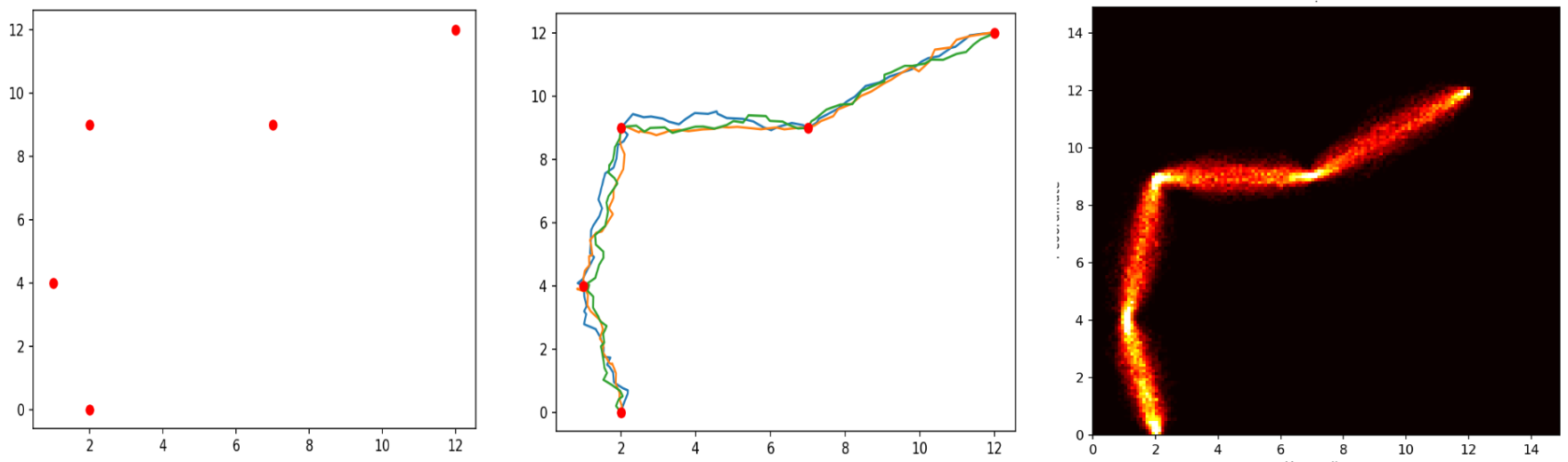
Luckily, I did have some code somewhat mapped out for this from my first week of investigating methods. Also, a lot of the data formatting code from the previous method was reusable. What we need to decide (and I'm about to cover how we do decide it) is what our ‘Brownian motion variance parameter’ is. This is a measure of how much the rangers wander between GPS points. Are we certain that from each GPS point they walk in a completely straight line to the next GPS point, or do we think that's the most likely path, but there might be some uncertainty as paths aren't always completely straight?
How we calculate this value (Laid out in this paper: link)
Basically, we can work out how straight the ranger's movement is by how straight the path is in general. For a point of GPS data (Zi), we look at the point before it (Zi-1), and the point after it (Zi+1) and ask ourselves ‘how close is Zi to the straight line that joins Zi-1, and Zi+1 We assume that the distance from Zi to this straight line will be normally distributed, and so we fit a standard deviation to this data.
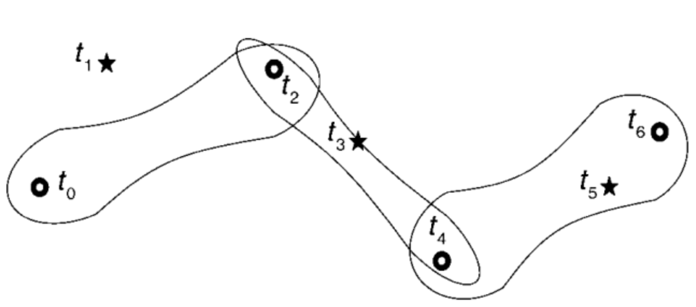
More formally: “consider the independent Brownian bridges on the nonoverlapping time intervals [t0, t2], [t2, t4], [t4, t6], ... , [tn-2, tn], while regarding the in-between observation times t1, t3, t5, ... , tn-1 as independent observations from these Brownian bridges”
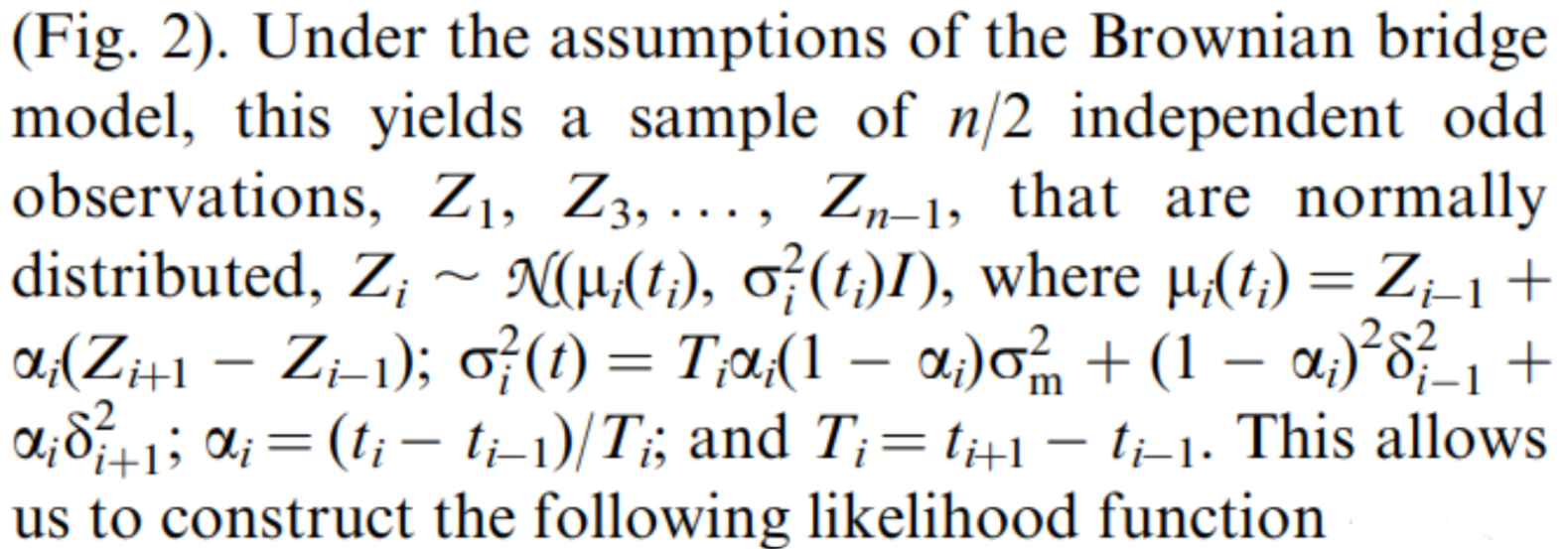

(delta is our measurement error, which we are assuming to be 0). Then, we find the maximum likelihood estimator of sigma m for this. This equation closely resembles the standard form of a normal distribution. However, one aspect puzzles me: I would have expected the first term to be the square root of its current value. I’m not sure why it appears as it does.
I used this method to find a value of variance for the model. I calculated a value of sigma for each path in the tracklog as some are straighter than others. Below are the results, on the left is a ranked version (using the ranking idea from the previous version) and on the right is the raw intensities (capped to reduce the effect of the long-tail distribution).
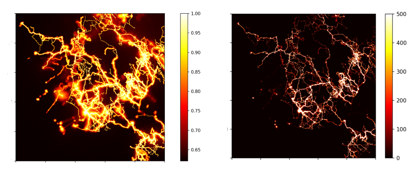
One thing I think we can see here is that there are some areas with very low but quite wide-reaching intensities (visible in the ranked version). The brownian bridge model is not sure exactly where the path is, and has guessed a low percentage over a large area. We need to consider how we handle this data, either using a cut-off, and just not considering anything below x percent, or using weighting in the model.
Speed has been implemented in a way similar to the method from before. Using the timestamps of GPS points, and for each pixel on the grid, taking the average. This is what the speed map looks like:
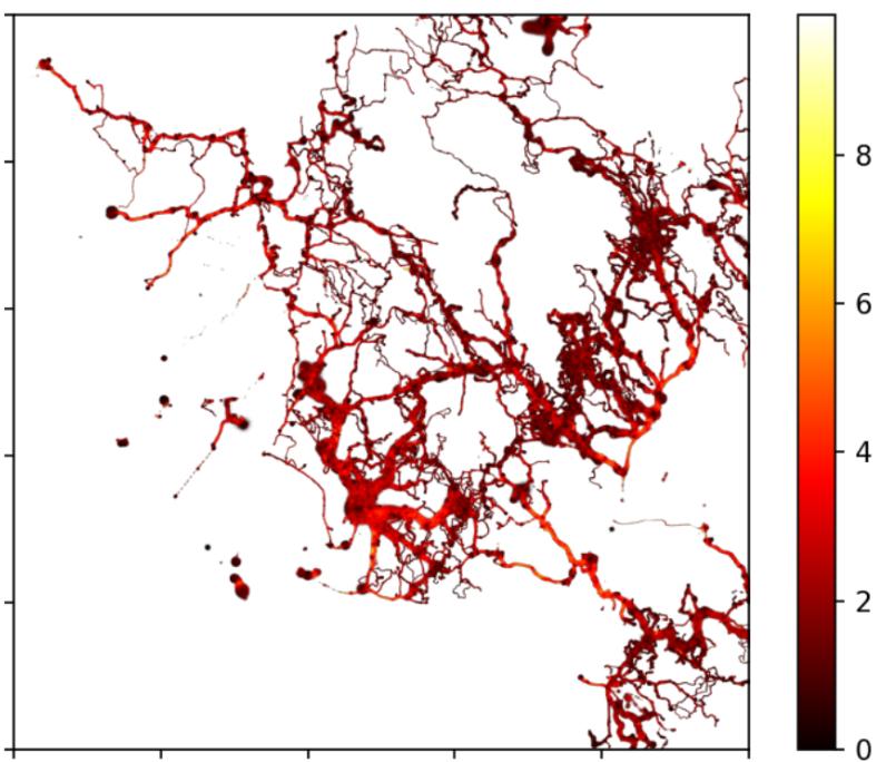
I have also employed the same tactic as before, of producing separate maps for north, south east and west. Gives us flexibility to investigate how slope affects speed.
This has now put me in a very similar position to where I was this time last week, but now with a different underlying model. I have the ranger data in map form and some preliminary feature data. I am back to running the machine learning models.